WORKED EXAMPLE · MONOTONIC RANK ASSOCIATION
Spearman Correlation Worked Example: Ordinal Severity and a Numeric Biomarker
Follow an ordinal imaging grade and numeric biomarker from paired participant-level data and a jittered scatterplot through tied ranks, Spearman’s correlation, interpretation, and BioTabular setup.
Published by BioTabularLast reviewed: November 2, 2026
This worked example uses synthetic data created for teaching. Imagine 25 independently sampled participants who each receive one ordered imaging-severity grade from 0 through 4 and one biomarker measurement. The scientific question is whether participants with higher severity grades generally have higher biomarker concentrations, without treating a one-grade step as a fixed numeric distance.
Define the paired variables and association target
- Observational unit
- One independently sampled participant.
- Pairing structure
- The severity grade and biomarker value on each row belong to the same participant.
- First variable
- Imaging-severity grade, ordered from 0 to 4.
- Second variable
- Biomarker concentration in ng/mL.
- Target
- The direction and strength of the population monotonic rank association.
- Starting method
- Two-sided Spearman rank correlation with average ranks for ties.
The values within a row form a meaningful pair, while the 25 participant rows are independent. Spearman correlation is symmetric: reversing the axes does not change the coefficient. The analysis does not designate one variable as a causal exposure and the other as an outcome.
Inspect the synthetic participant-level data
| Participant | Imaging-severity grade | Biomarker (ng/mL) |
|---|---|---|
| P01 | 0 | 2.3 |
| P02 | 0 | 3.1 |
| P03 | 0 | 2.8 |
| P04 | 0 | 4.0 |
| P05 | 0 | 3.5 |
| P06 | 1 | 2.9 |
| P07 | 1 | 4.4 |
| P08 | 1 | 3.7 |
| P09 | 1 | 5.1 |
| P10 | 1 | 3.3 |
| P11 | 2 | 3.8 |
| P12 | 2 | 5.6 |
| P13 | 2 | 4.7 |
| P14 | 2 | 6.2 |
| P15 | 2 | 5.0 |
| P16 | 3 | 5.1 |
| P17 | 3 | 7.4 |
| P18 | 3 | 6.3 |
| P19 | 3 | 8.5 |
| P20 | 3 | 5.8 |
| P21 | 4 | 7.0 |
| P22 | 4 | 9.2 |
| P23 | 4 | 8.1 |
| P24 | 4 | 12.0 |
| P25 | 4 | 10.4 |
Look at the paired observations before calculating a coefficient
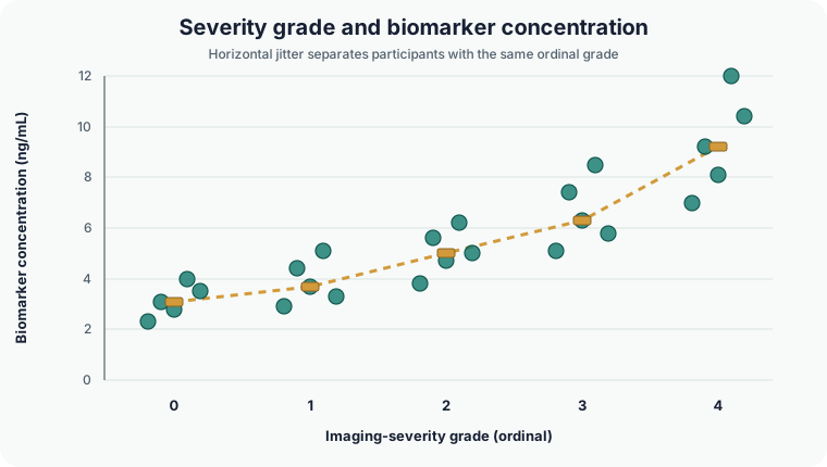
The points move upward overall as severity increases, but they form five vertical grade bands rather than a straight-line cloud. Adjacent grades overlap, and the rise is steeper at the upper end. This is a positive monotonic pattern: higher grades generally accompany higher concentrations, without requiring a constant increase for every one-grade step.
A U-shaped pattern would not be summarized well by Spearman correlation because its direction changes. A scatterplot remains essential even when the chosen calculation uses ranks.
Replace values with ranks and handle ties
Spearman’s coefficient is the Pearson correlation of the two rank variables. The smallest value receives rank 1, the next receives rank 2, and so on. Tied values receive their average rank.
Each imaging grade occurs five times. Grade 0 occupies pooled positions 1 through 5, so every grade-0 participant receives severity rank 3. Grade 1 receives average rank 8; grades 2, 3, and 4 receive average ranks 13, 18, and 23. The biomarker value 5.1 also occurs twice, so both observations receive biomarker rank 13.5.
| Imaging grade | Participants | Average severity rank | Median biomarker (ng/mL) |
|---|---|---|---|
| 0 | 5 | 3 | 3.1 |
| 1 | 5 | 8 | 3.7 |
| 2 | 5 | 13 | 5.0 |
| 3 | 5 | 18 | 6.3 |
| 4 | 5 | 23 | 9.2 |
Average ranks preserve tied observations rather than breaking ties arbitrarily. Because ties are present, BioTabular reports an asymptotic approximation for the p-value rather than an exact no-ties permutation calculation.
Calculate Spearman’s rank correlation
- Complete pairs
- 25; omitted 0
- Severity grades
- 0 through 4; five participants per grade
- Spearman correlation
- ρs = 0.9062308
- Direction
- Strong positive monotonic association
- Two-sided p-value
- 4.53 × 10⁻¹⁰
- Computation
- Asymptotic approximation; ties detected
ρs = Pearson correlation of the paired average ranksρs = .9062; p < .001
At α = .05, the result provides evidence against a population Spearman correlation of zero. The coefficient’s positive sign matches the upward ordering in the figure. Its magnitude describes how consistently the participant ranks move together; it does not mean that severity “explains 90.6%” of the biomarker or that a one-grade increase causes a particular concentration change.
BioTabular currently does not display a confidence interval for Spearman’s ρ. A study requiring interval estimation should prespecify and report an appropriate validated interval method rather than reusing Pearson’s Fisher-z interval automatically.
Why this is not simply “Pearson for non-normal data”
The method choice follows the scale and association target. Imaging severity is ordinal: grade 4 is more severe than grade 3, but the numerical distance between grades need not equal the distance between grades 1 and 0. The question also concerns monotonic ordering rather than a straight-line biomarker increase.
Separate normality tests on severity and biomarker would not decide this question. Spearman correlation is useful here because ranks represent the ordered scientific target. It is not a universal repair for outliers, dependence, confounding, or a non-monotonic relationship.
Assumptions and practical checks
- Independent participant rows: each participant contributes one pair. Repeated scans, bilateral measurements, families, or sites require a dependence-aware analysis.
- Meaningful ordering: higher imaging grades consistently represent greater severity.
- Monotonic target: the relationship moves in one overall direction over the observed range. Inspect the plot rather than inferring shape from ρ alone.
- Correct pairing: never sort the two columns separately; each biomarker must remain linked to the correct participant’s grade.
- Transparent ties: repeated grades are expected and receive average ranks. The inferential calculation must acknowledge ties.
- No dominating or erroneous observation: ranks can reduce sensitivity to raw spacing, but they do not make data errors, extreme observations, or separated subgroups irrelevant.
Reproduce the result in BioTabular
- Download the synthetic CSV and open the Spearman correlation calculator.
- Import the file. Keep
Participant_IDas the identifier, markImaging_Severity_Gradeas ordinal or numeric, and keepBiomarker_ng_mLnumeric. - Confirm the variable roles, then select
Imaging_Severity_Gradeas the first variable andBiomarker_ng_mLas the second. - Confirm Spearman correlation, the two-sided alternative, and α = .05.
- Run the analysis. Confirm 25 complete pairs, no omissions, ρs = .906, p < .001, and the message “asymptotic approximation; ties detected.”
- Inspect the scatterplot and send it to Plot Studio. Preserve the grade bands and visible points; any horizontal jitter used for presentation must be labelled and must not alter the calculation.
Interpret and report the result
Within the observed grades and biomarker range, participants with higher imaging severity tend to have higher biomarker concentrations. The result concerns the ordering of participant pairs. It does not estimate the biomarker difference between grades, identify a diagnostic threshold, demonstrate agreement between measurements, or show that severity causes biomarker change.
“Among 25 independent participants with complete measurements, imaging-severity grade and biomarker concentration showed a strong positive monotonic association (Spearman ρs = .906, two-sided p < .001). Tied imaging grades were assigned average ranks and an asymptotic p-value was used. The jittered scatterplot showed increasing biomarker concentrations across ordered grades with overlap between adjacent grades.”
A complete study report should also define the grading system, measurement timing, participant selection, missing-pair handling, whether the analysis was prespecified, and any sensitivity analyses for important subgroups or unusual observations.
Common mistakes this example avoids
- Treating an ordinal grade as if every one-unit step had equal quantitative meaning.
- Choosing Spearman only because a separate normality test was significant.
- Calculating a coefficient without inspecting the paired observations.
- Breaking participant pairing by sorting columns independently.
- Calling a monotonic coefficient a fitted curve or a per-grade effect.
- Interpreting a strong correlation as causation, agreement, discrimination, or clinical usefulness.
- Treating repeated participant measurements as independent pairs.
Limits of this worked example
The dataset is small, complete, synthetic, and intentionally monotonic. It has balanced counts at each grade, no covariates, repeated measurements, clusters, missing pairs, verification bias, or prespecified clinical threshold. Real studies may need ordinal regression, nonlinear regression, partial association, repeated-measures methods, multilevel models, measurement-error analysis, diagnostic-accuracy analysis, or multiplicity control when many correlations are screened.
Related resources
Read Pearson vs. Spearman Correlation for the broader method choice. Compare this monotonic rank target with the Pearson correlation worked example, which summarizes an approximately linear association between two numeric variables. Return to Which Statistical Test Should I Use? for other data structures.
References and further reading
- R documentation: Test for association between paired samples
- Spearman (1904): The proof and measurement of association between two things
- BMJ Statistics Notes: Correlation and regression
- NIST/SEMATECH e-Handbook of Statistical Methods
- American Statistical Association statement on statistical significance and p-values
BioTabular’s editorial approach and scope explain how these educational resources are prepared and what they do not replace.