STUDYING ASSOCIATIONS
Pearson vs. Spearman Correlation: Which Measure of Association Should You Use?
Use Pearson correlation when a linear association is the target and the scatterplot supports that description. Use Spearman correlation when a monotonic, rank-based association is the target. Before calculating either statistic, inspect the scatterplot.
Published by BioTabularLast reviewed: August 18, 2026
Pearson and Spearman correlation both describe how two variables vary together. The right choice depends mainly on the pattern visible in the data and the question being asked—not on a rule that one method is always safer than the other.
A single correlation coefficient cannot reveal curvature, outliers, clusters, restricted ranges, or repeated measurements from the same unit.
The short answer
| Question or data pattern | Usual starting point |
|---|---|
| How strongly do two numeric variables follow a straight-line pattern? | Pearson correlation (r) |
| Do larger values of one variable tend to go with larger or smaller values of the other, even if the pattern is curved? | Spearman rank correlation (ρ or rs) |
| Is one or both variables ordinal? | Spearman correlation is often appropriate |
| Is the scatterplot U-shaped or otherwise non-monotonic? | Neither correlation alone summarizes the relationship well; model or describe the pattern directly |
| Are many observations repeated within the same person, sample, site, or experiment? | Use a method that accounts for clustering or repeated measures; an ordinary correlation treats observations as independent |
The choice is about the relationship to summarize. It is not a contest between a “parametric” method and a universally assumption-free alternative.
What Pearson correlation measures
Pearson’s correlation coefficient, usually written r, measures the strength and direction of a linear association between two numeric variables. It ranges from −1 to +1.
- r near +1 indicates a strong positive linear pattern: larger values of one variable tend to occur with larger values of the other.
- r near −1 indicates a strong negative linear pattern: larger values of one variable tend to occur with smaller values of the other.
- r near 0 indicates little or no linear association. It does not prove that the variables have no relationship.
Pearson correlation is calculated from the original values. It is useful when a straight-line summary is meaningful—for example, when examining the association between two continuous laboratory measurements over the range observed.
Example: two quantitative measurements
Suppose researchers collect one blood sample from each of 80 independent participants and measure two distinct biomarkers in each sample. Each plotted point pairs the two biomarker values from one participant; the 80 participant-level pairs should be independent of one another. If the scatterplot shows points spread around an upward-sloping straight line, with no single point dominating the pattern, Pearson correlation can summarize the linear association between the biomarkers.
The result describes association, not agreement or interchangeability. Two methods can be strongly correlated while having a consistent offset or clinically important differences. Method-comparison questions often need an agreement analysis, such as a Bland–Altman approach, rather than correlation alone.
What Spearman correlation measures
Spearman correlation, commonly written ρ (rho) or rs, is the Pearson correlation calculated after replacing each variable’s values with their ranks. It measures the strength and direction of a monotonic association.
Like Pearson’s r, Spearman’s ρ ranges from −1 to +1. Values near +1 indicate a strong positive monotonic association, values near −1 indicate a strong negative monotonic association, and values near 0 indicate little or no monotonic association.
A relationship is monotonic when it moves in one overall direction: as one variable increases, the other generally increases or generally decreases. The pattern does not have to be a straight line. For example, a curve that rises quickly and then levels off can still be monotonic.
Because Spearman uses ranks, the exact spacing between values matters less than their order. This makes it particularly useful for ordered categories and for numeric data where a monotonic rank-based summary better matches the question. Tied values receive appropriate average ranks in standard implementations.
Example: an ordered rating and a biomarker
Suppose symptom severity is recorded on an ordered five-level scale and a biomarker is measured continuously. If higher severity categories generally correspond to higher biomarker values, Spearman correlation can summarize that ordered association. A scatterplot with jitter, or a plot of the biomarker distribution by rating, should still accompany the statistic.
Linear is not the same as monotonic
This distinction is the heart of the choice.
| Pattern in a scatterplot | Pearson correlation | Spearman correlation |
|---|---|---|
| Points follow an upward or downward straight-line cloud | Directly summarizes the pattern | Also may be high, but discards distance information |
| Values rise quickly then level off, while always moving upward overall | Can understate the strength of the curved pattern | Often provides a useful monotonic summary |
| U-shaped or inverted-U pattern | May be near zero despite a clear relationship | May also be near zero because the direction changes |
| One extreme observation drives the apparent trend | Can change substantially | May be less affected, but the observation still needs investigation |
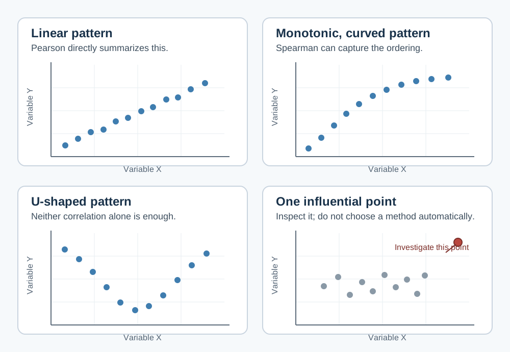
Neither coefficient replaces looking at the plot. A U-shaped relationship can produce a correlation close to zero even when the variables are clearly related. In that situation, consider a scientifically justified nonlinear model, a transformed scale, or a descriptive figure rather than presenting a single correlation as the answer.
Start with the study design and a scatterplot
For each row, ask whether the two values form one meaningful pair—for example, a participant’s exposure and outcome measured once, or two different biomarkers measured from one sample. The two values within a row are deliberately paired because correlation describes their association; the rows, or participant-level pairs, should ordinarily be independent of one another. Then inspect the scatterplot before choosing a coefficient.
Look for:
- Whether the direction is roughly straight-line, monotonic but curved, or non-monotonic.
- Outliers or influential observations.
- Clusters that may represent different groups, sites, batches, or conditions.
- A narrow observed range, which can make a correlation look weaker than it would in a broader population.
- Many repeated values, especially for ordinal or rounded variables.
- Repeated observations from the same participant, animal, specimen, or site.
If a few points look surprising, first check for data-entry, unit, or measurement issues. Do not remove observations merely because they reduce a desired correlation. If they are valid observations, show their influence through a plot and explain how they were handled.
Common misconceptions
“Spearman is Pearson correlation for non-normal data.”
Not quite. The choice should not be based only on whether a normality test is significant. Pearson correlation describes a linear relationship; Spearman describes a monotonic rank relationship. The scatterplot, measurement scale, scientific question, sample size, and influence of unusual observations are more informative than a mechanical normality-test rule.
For confidence intervals and p-values, the sampling assumptions and method of inference still matter. With small samples, strong skewness, influential observations, or complex designs, consider a suitable resampling or model-based approach and seek statistical advice when needed.
“Spearman has no assumptions.”
Spearman makes fewer demands about the values’ original scale, but it still needs a meaningful paired structure and an interpretable monotonic relationship for its usual interpretation. Ordinary correlation calculations also generally treat the rows as independent. Correlating repeated measurements as though they came from different people or samples can understate uncertainty.
“A statistically significant correlation is important.”
Not necessarily. With a large sample, a very small association can have a small p-value. Report the coefficient and confidence interval, inspect the plot, and consider whether the magnitude is scientifically or clinically meaningful.
“A non-significant correlation means there is no relationship.”
No. It may reflect limited precision, a restricted range, an unmeasured nonlinear pattern, or an effect that is smaller than the study can distinguish from zero. A confidence interval communicates the range of linear or monotonic associations compatible with the data and analysis.
“Correlation shows causation.”
No. A correlation does not establish that one variable causes the other. Confounding, reverse causation, selection, shared measurement processes, and chance can all create associations. Causal questions need a design and analysis that address those alternatives.
When ordinary correlation is not enough
Ordinary Pearson or Spearman correlation is most straightforward when each row is an independent pair of measurements. Use additional methods when the data structure is more complex.
- Repeated measures: Multiple observations from the same unit need a repeated-measures, multilevel, or otherwise clustered analysis.
- Groups or confounders: A relationship can differ by treatment group, site, or another variable. Stratified plots or an appropriate regression model may be clearer than one pooled correlation.
- Time series: Measurements close in time can be correlated because of trends or autocorrelation. Analyze the time structure rather than treating every time point as independent.
- Binary, nominal, or count outcomes: A correlation coefficient may not be the most meaningful summary; use a method suited to the outcome and research question.
- Agreement between measurement methods: Correlation alone does not measure agreement. Assess bias and limits of agreement as well.
What to report
For a correlation analysis, report:
- The variables, units, population, and number of complete paired observations.
- Whether Pearson or Spearman correlation was used and why.
- The coefficient, its confidence interval, and p-value when inferential reporting is appropriate.
- A scatterplot that shows the data, with a fitted line or smooth only when clearly labelled and useful.
- How outliers, ties, missing paired values, repeated measures, and any transformations were handled.
For example: “Among 84 complete participant pairs, the biomarker and symptom score showed a positive Spearman correlation (ρ = 0.46, 95% CI 0.27 to 0.61, p < .001). The scatterplot suggested a monotonic, non-linear pattern.” The exact confidence-interval method should be appropriate for the study and stated when relevant.
When to seek additional statistical support
Consult a statistician before analysis when observations are clustered or repeated, when a correlation will support a causal or clinical decision, when substantial missingness or selection is present, when several correlations are being screened, or when the relationship may be nonlinear, time-dependent, or confounded. The analysis should follow the study question and design rather than selecting the coefficient with the most favorable result.
Related resources
For a broader path through common statistical methods, see Which Statistical Test Should I Use?. For a study-design distinction that also affects analysis, see Paired vs. Independent Samples: How Study Design Changes Your Statistical Test. For choosing a test for two categorical variables, read Chi-square vs. Fisher’s Exact Test: How to Choose for Categorical Data. For an introduction to distributional shape and diagnostics, read What Is a Normal Distribution? A Practical Guide for Research Data.
References and further reading
- NIST/SEMATECH e-Handbook of Statistical Methods
- American Statistical Association statement on statistical significance and p-values
BioTabular’s editorial approach and scope explain how these educational resources are prepared and what they do not replace.