WORKED EXAMPLE · REPEATED MEASUREMENTS
Longitudinal Mixed-Model Worked Example: Repeated Outcomes Over Time
Follow repeated symptom scores from long-format data and a missing visit through a random-intercept linear mixed model, treatment-by-time interaction, fitted trajectories, and reporting.
Published by BioTabularLast reviewed: October 29, 2026
This worked example uses synthetic data created for teaching. Imagine a twelve-week randomized study in which eight participants receive treatment and eight receive control. Symptom scores are scheduled at baseline and weeks 4, 8, and 12. Lower scores indicate fewer symptoms. Because measurements from the same participant are correlated, treating all 64 scheduled rows as independent would understate uncertainty.
Define the design and the target
- Observational unit
- The participant; each participant contributes measurements at repeated time points.
- Analysis data structure
- The downloadable file is in long format, with one row per participant and visit. The table below displays the same values in wide format for easier reading.
- Outcome
- A continuous symptom score for which lower values are better.
- Time
- Study week coded numerically as 0, 4, 8, and 12.
- Primary target
- The treatment-versus-control difference in the linear rate of symptom change.
- Starting method
- A random-intercept linear mixed model with group, time, and group-by-time fixed effects.
The interaction is the central term. It asks whether the expected rate of change differs between groups. It is not the treatment-versus-control difference at week 12, and it is not the within-treatment change by itself.
Inspect the synthetic repeated measurements
The table presents one participant per row and one visit per measurement column so the repeated profiles are easy to compare. This is a wide display; it is not the layout of the downloadable analysis file.
| Participant | Group | Week 0 | Week 4 | Week 8 | Week 12 |
|---|---|---|---|---|---|
| C01 | Control | 52 | 50 | 52 | 49 |
| C02 | Control | 48 | 50 | 47 | 48 |
| C03 | Control | 55 | 53 | 55 | 52 |
| C04 | Control | 50 | 51 | 48 | 50 |
| C05 | Control | 53 | 51 | 53 | 50 |
| C06 | Control | 47 | 49 | 46 | 47 |
| C07 | Control | 56 | 54 | 56 | 53 |
| C08 | Control | 49 | 50 | 47 | 49 |
| T01 | Treatment | 52 | 49 | 47 | 42 |
| T02 | Treatment | 49 | 48 | 42 | 41 |
| T03 | Treatment | 55 | 51 | 50 | 44 |
| T04 | Treatment | 50 | 49 | — | 40 |
| T05 | Treatment | 53 | 49 | 49 | 43 |
| T06 | Treatment | 47 | 47 | 40 | 39 |
| T07 | Treatment | 56 | 51 | 52 | 45 |
| T08 | Treatment | 49 | 48 | 42 | 42 |
In the downloadable long-format file, these 16 participant rows become 64 participant-visit rows: each participant appears once for each scheduled visit. Participant T04 has no week-8 outcome. BioTabular omits that incomplete participant-visit row but retains T04’s other three measurements, leaving 63 included observations from 16 participants.
Plot individual profiles before fitting the model
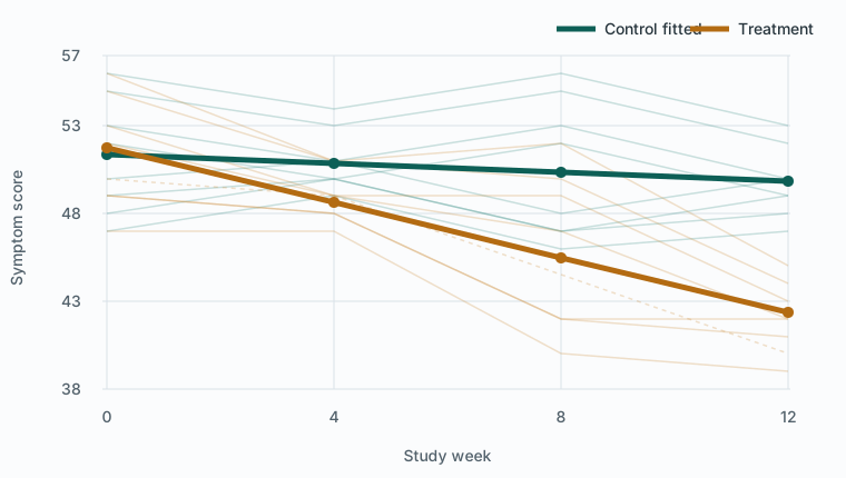
The plot makes the dependence visible: four measurements from one participant form a profile, not four independent people. It also shows considerable between-participant variation in baseline score and an approximately linear average trend over the four scheduled times. A visibly curved trajectory would call for a different time specification, such as categorical time or a justified nonlinear term.
Specify the random-intercept model
With Control as the reference group and week 0 as time zero, the fitted model is:
Score = β₀ + β₁(week) + β₂(treatment) + β₃(week × treatment) + participant intercept + residualPrimary term: β₃, the treatment-versus-control difference in weekly slopes
The participant-specific random intercept allows people to begin above or below the population trajectory while assuming a common fixed slope within each group. Time is entered in weeks, so every slope coefficient is interpreted per one week. Coding time as 0, 4, 8, and 12 also makes the intercept and treatment main effect refer to baseline.
BioTabular fits this random-intercept model by maximum likelihood and reports Wald normal-approximation intervals and p-values for the fixed coefficients. The model is intentionally focused: it does not fit random slopes, nonlinear time, covariates, site effects, or alternative residual-correlation structures.
Read the fixed-effect coefficients in context
| Term | Estimate | 95% CI | p | Meaning under this coding |
|---|---|---|---|---|
| Intercept | 51.375 | 49.538 to 53.212 | < .001 | Fitted control mean at week 0 |
| Time | −0.125 | −0.229 to −0.021 | .018 | Control change per week |
| Treatment | 0.367 | −2.231 to 2.965 | .782 | Treatment minus control at week 0 |
| Time × treatment | −0.658 | −0.805 to −0.511 | < .001 | Additional weekly change in treatment versus control |
- Included data
- 63 observations from 16 participants
- Omitted data
- 1 missing outcome row
- Control slope
- −0.1250 points per week
- Treatment slope
- −0.7832 points per week
- Slope difference
- −0.6582 points per week
- 95% CI for slope difference
- −0.8054 to −0.5111
The treatment slope is obtained by adding the time and interaction coefficients: −0.1250 + (−0.6582) = −0.7832 points per week. Over twelve weeks, the fitted control change is −1.50 points and the fitted treatment change is about −9.40 points. Their difference in change is about −7.90 points.
The fitted week-12 means are 49.875 for control and 42.343 for treatment, a difference of −7.532 points. That week-12 difference combines the small fitted baseline difference with twelve weeks of slope separation; it is not numerically identical to the interaction coefficient.
Understand the random intercept and ICC
- Random-intercept variance
- 5.768
- Residual variance
- 1.796
- Intraclass correlation
- 0.763
- Estimation
- Maximum likelihood
The estimated intraclass correlation indicates that repeated observations from the same participant are strongly related under this model. It is a model-based variance summary, not a reliability certificate and not proof that the chosen covariance structure is correct. The high value reinforces why an ordinary independent-observations analysis would be unsuitable.
Reproduce the analysis in BioTabular
- Download the synthetic CSV and open the longitudinal mixed-model calculator.
- Import the file. Mark
Participant_IDas the ID,Groupas categorical, and bothWeekandSymptom_Scoreas numeric. - Review the group order and keep Control before Treatment so the coefficients use Control as the reference.
- Confirm the variable roles. Choose
Participant_ID,Group,Week, andSymptom_Scorefor the corresponding model fields. - Run the model at α = .05. Confirm 63 included observations, one omitted row, 16 participants, and an interaction estimate of −0.658 with a 95% interval from −0.805 to −0.511.
- Inspect the longitudinal figure and the participant profiles. Do not interpret the interaction from the coefficient table without confirming that the time scale and trajectory shape are meaningful.
Interpret and report the result
The synthetic study supports different average linear symptom trajectories between groups. Treatment participants are estimated to improve faster, because their symptom scores decline about 0.66 points per week more than control. The baseline treatment coefficient is small and imprecise, but a nonsignificant baseline coefficient is neither required for randomization nor evidence that the groups are identical.
“A maximum-likelihood random-intercept linear mixed model included treatment group, study week, and their interaction. Sixty-three observations from 16 participants were analyzed; one scheduled outcome was missing. The treatment-by-week interaction was −0.658 symptom-score points per week (95% CI −0.805 to −0.511; Wald z = −8.77, p < .001), indicating a faster decline in the treatment group. The fitted weekly slope was −0.125 points for control and −0.783 points for treatment. The estimated random-intercept variance was 5.768, residual variance was 1.796, and intraclass correlation was .763.”
If treatment was randomly assigned and the analysis plan and missing-data assumptions are defensible, the interaction can support a treatment-effect interpretation. In an observational study, the same coefficient describes adjusted trajectory differences under the specified model; it does not remove confounding merely because a mixed model was used.
Missing data require an assumption, not just software
Retaining T04’s observed visits is an advantage over discarding the entire participant, but the model does not make the missing week-8 value harmless. Likelihood-based inference is commonly interpreted under assumptions about the missing-data process, including that missingness is explainable from observed information under a missing-at-random framework. Researchers should report the amount and pattern of missingness, investigate why visits were missed, and plan sensitivity analyses when departures could change the conclusion.
Common mistakes this example avoids
- Running a separate t-test at every visit and treating the collection of p-values as one longitudinal analysis.
- Treating all measurement rows as independent participants.
- Calling the treatment main effect the overall treatment effect when time zero is baseline.
- Interpreting the interaction as the week-12 group difference.
- Changing the unit of time without recognizing that the slope coefficients change scale.
- Assuming a random intercept automatically handles nonlinear trajectories, random slopes, informative dropout, clustering by site, or baseline imbalance.
- Reporting only p-values without fitted slopes, confidence intervals, trajectories, and missing-data information.
Limits of this worked example
The dataset is small, synthetic, and deliberately follows approximately linear group trajectories. It has one missing outcome, no covariates, one level of clustering, and equal planned visit times. Real studies may need categorical or nonlinear time, random slopes, small-sample degrees-of-freedom corrections, additional covariance structures, baseline adjustment chosen for the design, site or family effects, heterogeneous residual variance, or a prespecified missing-data sensitivity analysis. Consult a statistician for confirmatory or regulated longitudinal analyses.
Related resources
Compare this multi-visit design with the paired t-test before-and-after worked example, which has exactly two complete measurements per participant and asks about a mean within-person difference. Return to Paired vs. Independent Samples for the broader design distinction, or use Which Statistical Test Should I Use? for other outcome structures.
References and further reading
- lme4 vignette: Fitting linear mixed-effects models
- lme4 documentation: Fit linear mixed-effects models
- NIST/SEMATECH e-Handbook of Statistical Methods
- American Statistical Association statement on statistical significance and p-values
BioTabular’s editorial approach and scope explain how these educational resources are prepared and what they do not replace.