WORKED EXAMPLE
Paired T-Test Worked Example: Before-and-After Measurements
Follow a paired t-test from a participant-level before-and-after dataset through the within-person differences, assumptions, calculation, confidence interval, BioTabular setup, interpretation, and reporting language.
Published by BioTabularPublished and reviewed: October 21, 2026
This example is a complete teaching pathway, not clinical evidence. The values are synthetic, and the result does not establish that a real intervention lowers blood pressure.
Research question and study design
Suppose a pilot study measures systolic blood pressure immediately before an intervention and again eight weeks later in the same 12 participants. The research question is: What is the mean within-participant change in systolic blood pressure from before to after the intervention?
- Observational unit
- The participant.
- Pairing key
- Participant ID links each person’s before and after values.
- Outcome
- Systolic blood pressure in millimetres of mercury (mmHg).
- Estimand
- The population mean within-participant change after eight weeks.
- Subtraction direction
- After minus before. Negative differences represent lower blood pressure after eight weeks.
- Starting method
- A two-sided paired t-test when a mean change is scientifically meaningful and the assumptions are reasonable.
The synthetic before-and-after dataset
Every row is one participant and every difference is calculated in the same direction. Participant P08 increased by 1 mmHg, so the data do not imply that every individual improved.
| Participant | Before (mmHg) | After (mmHg) | Change: after − before (mmHg) |
|---|---|---|---|
| P01 | 142 | 136 | −6 |
| P02 | 135 | 131 | −4 |
| P03 | 151 | 144 | −7 |
| P04 | 128 | 127 | −1 |
| P05 | 146 | 141 | −5 |
| P06 | 139 | 131 | −8 |
| P07 | 132 | 129 | −3 |
| P08 | 144 | 145 | +1 |
| P09 | 137 | 133 | −4 |
| P10 | 149 | 143 | −6 |
| P11 | 130 | 128 | −2 |
| P12 | 141 | 136 | −5 |
Privacy note: this downloadable file is synthetic. When it is imported into the Workspace, BioTabular processes it in browser memory during the active page session rather than uploading the rows to BioTabular.
Why the analysis is paired
P01’s after value belongs with P01’s before value, not with another participant’s baseline value. The participant identifier and study design create that link. The analysis therefore reduces the two measurement columns to one sample of 12 within-participant differences.
An independent two-sample test would discard these links and answer a different question about two marginal groups of measurements. The fact that both columns contain 12 values is not sufficient by itself; the meaningful, verified one-to-one correspondence is what makes the data paired.
Calculate the paired t-test
For participant i, define di = afteri − beforei. The paired t-test is a one-sample t-test of whether the population mean of these differences is zero.
- Complete pairs
- 12
- Mean before
- 139.50 mmHg
- Mean after
- 135.33 mmHg
- Mean difference
- −4.1667 mmHg
- SD of differences
- 2.5878 mmHg
- Standard error
- 0.7470 mmHg
t = mean difference ÷ standard error−4.1667 ÷ 0.7470 = −5.5775
With 12 complete pairs, the degrees of freedom are 11. The two-sided p-value is 0.0001658. The 95% confidence interval for after minus before is −5.8109 to −2.5224 mmHg.
Inspect the individual changes
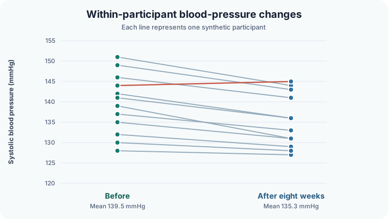
The connected values reveal variation hidden by the two means. Most participants decreased, one changed little, and P08 increased slightly. This does not invalidate the paired t-test, but it is a reminder to interpret the estimated average alongside the observed individual data.
Assumptions and practical checks
The paired t-test does not require the before and after columns to be normally distributed separately. Its mean-based inference concerns the distribution of the within-participant differences.
- Correct pairs: verify every pair with the participant ID rather than relying on row position alone.
- Independent participants: one participant’s difference should not determine another participant’s difference.
- Numeric outcome and meaningful mean: the measurement scale must support a mean difference interpretation.
- Difference distribution: inspect the 12 differences for data errors, strong skewness, or an influential outlier.
- Complete-pair handling: state how missing baseline or follow-up values were handled.
This dataset has 12 complete pairs and no missing values. In real research, do not delete an unusual difference merely because it changes the p-value. Check the source record, show the observed data, and use a sensitivity analysis or a different prespecified method when justified.
Reproduce the result in BioTabular
- Download the synthetic CSV and open the BioTabular t-test calculator.
- Import the file. Keep
Participant_IDas the identifier and the measurement fields as numeric variables. - Choose Paired t-test.
- Set First measurement to
After_mmHgand Second measurement toBefore_mmHg. BioTabular reports first minus second, reproducing after minus before. - Keep the two-sided alternative and 0.05 significance level for this example, then run the analysis.
- Confirm that the output reports 12 complete pairs and 0 omitted pairs. Use the paired dot-and-line Plot Studio handoff to inspect the individual trajectories.
Interpret the result
The estimated mean after-minus-before change is −4.17 mmHg. Under the paired t-test model, the synthetic data are compatible with an average decrease of roughly 2.5 to 5.8 mmHg. The confidence interval quantifies uncertainty around the mean change; it is not a range expected to contain 95% of individual changes.
The small p-value describes how incompatible the observed mean difference is with a zero population mean difference under the model. It does not establish clinical importance, prove that the intervention caused the change, or imply that every participant’s blood pressure decreased.
Reporting example
“Systolic blood pressure was lower after eight weeks than before the intervention (mean within-participant change, after minus before: −4.17 mmHg; 95% CI −5.81 to −2.52; paired t(11) = −5.58; two-sided p < .001; 12 complete pairs).”
A full study report should also name the intervention, population, measurement schedule, missing-data handling, and whether the analysis was prespecified.
Common mistakes this example avoids
- Treating the before and after values as independent groups.
- Reversing the subtraction direction while keeping an interpretation written for the other direction.
- Checking only the original columns rather than examining the paired differences.
- Reporting only p < .001 without the mean change and confidence interval.
- Drawing lines between values that were not verified with a participant ID.
- Interpreting the average decrease as proof that every participant improved.
Limits of this worked example
This illustration has two time points, one complete pair per participant, no comparison group, and no covariate adjustment. A pre/post change alone cannot separate an intervention effect from time trends, regression to the mean, measurement variation, or other causes. Three or more time points, incomplete follow-up, clustering, or a treatment-by-time question may require a repeated-measures or mixed-effects model.
Related resources
Return to Paired vs. Independent Samples for the broader study-design decision. For a general route through common methods, see Which Statistical Test Should I Use?.
References and further reading
- NIST/SEMATECH: Analysis of paired observations
- Statistics review 5: Comparison of means
- The differences and similarities between two-sample and paired t-tests
- NIST/SEMATECH e-Handbook of Statistical Methods
- American Statistical Association statement on statistical significance and p-values
BioTabular’s editorial approach and scope explain how these educational resources are prepared and what they do not replace.