WORKED EXAMPLE · ORDINAL OUTCOMES ACROSS THREE GROUPS
Kruskal–Wallis and Dunn Worked Example: Ordinal Scores Across Three Independent Groups
Follow tied ordinal pain-interference scores through a rank-based three-group comparison, tie correction, Holm-adjusted Dunn follow-ups, interpretation, and BioTabular setup.
Published by BioTabularLast reviewed: November 1, 2026
This worked example uses synthetic data created for teaching. Imagine a randomized three-arm study in which each participant is assigned to control, a standard program, or an intensive program. At week 6, each participant reports pain interference on an ordered scale from 0 to 10, where lower values indicate less interference. Every participant contributes one score.
Define the design and the rank-based question
- Observational unit
- One independently randomized participant.
- Groups
- Control, standard program, or intensive program; each participant belongs to one group only.
- Outcome
- Week-6 pain-interference score from 0 to 10, treated as an ordered outcome.
- Primary question
- Are the population score distributions equal across all three groups?
- Follow-up question
- Which group pairs differ after accounting for the three pairwise comparisons?
- Starting method
- A tie-corrected Kruskal–Wallis test followed by two-sided Dunn comparisons with Holm adjustment.
The null hypothesis is that the three population distributions are equal. The alternative is that at least one differs. This is a rank-distribution question—not the same estimand as the mean comparison in one-way ANOVA. A location or median interpretation requires additional context about the shapes and spreads of the group distributions.
Inspect the synthetic participant-level data
The file contains 36 complete observations, with 12 independent participants in each group. Scores repeat because this integer scale has eleven possible categories—0 through 10 inclusive. That count is unrelated to the test’s degrees of freedom. BioTabular assigns average ranks to tied observations and applies the standard tie correction.
| Participant | Program | Pain-interference score |
|---|---|---|
| C01 | Control | 8 |
| C02 | Control | 7 |
| C03 | Control | 9 |
| C04 | Control | 6 |
| C05 | Control | 8 |
| C06 | Control | 7 |
| C07 | Control | 9 |
| C08 | Control | 8 |
| C09 | Control | 6 |
| C10 | Control | 7 |
| C11 | Control | 8 |
| C12 | Control | 9 |
| S01 | Standard program | 6 |
| S02 | Standard program | 5 |
| S03 | Standard program | 7 |
| S04 | Standard program | 6 |
| S05 | Standard program | 5 |
| S06 | Standard program | 6 |
| S07 | Standard program | 7 |
| S08 | Standard program | 5 |
| S09 | Standard program | 6 |
| S10 | Standard program | 4 |
| S11 | Standard program | 7 |
| S12 | Standard program | 6 |
| I01 | Intensive program | 5 |
| I02 | Intensive program | 4 |
| I03 | Intensive program | 6 |
| I04 | Intensive program | 5 |
| I05 | Intensive program | 3 |
| I06 | Intensive program | 4 |
| I07 | Intensive program | 6 |
| I08 | Intensive program | 5 |
| I09 | Intensive program | 4 |
| I10 | Intensive program | 3 |
| I11 | Intensive program | 5 |
| I12 | Intensive program | 6 |
Describe the observed score distributions
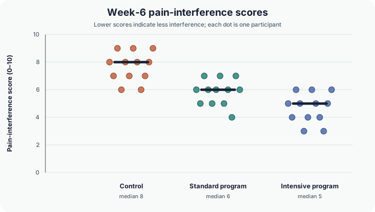
- Control
- n = 12; median = 8; IQR = 1.25; mean rank = 28.9583
- Standard program
- n = 12; median = 6; IQR = 1.25; mean rank = 17.2083
- Intensive program
- n = 12; median = 5; IQR = 1.25; mean rank = 9.3333
- Complete observations
- 36 included; 0 omitted
- Observed scores
- 3 through 9, with ties at every value
- Direction
- Lower ranks correspond to less pain interference
Calculate the tie-corrected Kruskal–Wallis statistic
All 36 scores are pooled and ranked from smallest to largest. Tied scores receive their average rank. The test compares each group’s rank sum with what would be expected if the group distributions were equal, then corrects the statistic for ties.
A mean rank is the sum of a group’s pooled ranks divided by that group’s sample size. For example, the two scores of 3 occupy pooled ranks 1 and 2, so each receives rank 1.5. The four scores of 4 occupy ranks 3 through 6, so each receives rank 4.5. The complete pooled ranking is:
| Observed score | Pooled count | Average rank assigned |
|---|---|---|
| 3 | 2 | 1.5 |
| 4 | 4 | 4.5 |
| 5 | 7 | 10.0 |
| 6 | 10 | 18.5 |
| 7 | 6 | 26.5 |
| 8 | 4 | 31.5 |
| 9 | 3 | 35.0 |
The control participants’ ranks sum to 347.5, so their mean rank is 347.5 ÷ 12 = 28.9583. The standard-program rank sum is 206.5, giving 17.2083. The intensive-program rank sum is 112.0, giving 9.3333. Because lower scores receive lower ranks, the intensive group has the lowest mean rank. These are summaries of pooled ranks, not means of the original 0–10 scores.
H = tie-corrected contrast among the three group rank sumsH(2) = 21.8803; p = 0.0000177
The degrees of freedom are the number of groups minus one: 3 − 1 = 2. At α = .05, the result provides evidence that at least one population score distribution differs. It does not identify which pair differs, prove that all pairs differ, or estimate a mean difference. The low p-value also does not measure clinical importance.
Follow the omnibus result with Holm-adjusted Dunn comparisons
Dunn comparisons use differences in mean ranks and the same tie-aware rank variance as the overall analysis. Holm adjustment controls the family-wise error rate across the three pairwise tests without assuming that an unadjusted p-value can be read in isolation. The contrast is the second named group minus the first, so negative z values indicate lower ranks in the program group.
| Contrast | z | Raw p | Holm-adjusted p |
|---|---|---|---|
| Standard program − Control | −2.7826 | 0.00539 | 0.01079 |
| Intensive program − Control | −4.6475 | 0.00000336 | 0.0000101 |
| Intensive program − Standard program | −1.8649 | 0.06219 | 0.06219 |
Assumptions and design checks
- Independent observations: each participant contributes one score to one group. Repeated, matched, family-clustered, or site-clustered observations need a method that represents that dependence.
- Ordered outcome: larger values consistently mean more pain interference, so ranking is meaningful.
- Comparable measurement: all groups use the same scale, timing, instructions, and scoring rule.
- Distributional interpretation: Kruskal–Wallis tests equality of distributions. Describing a location shift or median difference requires that the shapes and spreads make that interpretation reasonable.
- Ties: repeated ordinal scores are expected. The calculation must use average ranks and a tie correction.
- Planned multiplicity control: pairwise questions and the Holm adjustment should be chosen from the analysis plan, not selected after viewing favorable comparisons.
Reproduce the result in BioTabular
- Download the synthetic CSV and open the Kruskal–Wallis calculator.
- Import the file. Keep
Participant_IDas the identifier,Programas categorical, andPain_Interference_Scoreas numeric or ordinal. - Review the group order as Control, Standard program, Intensive program, then confirm the variable roles.
- Choose outcome-plus-grouping-column format. Select
Pain_Interference_Scoreas the outcome andProgramas the grouping column. - Keep Holm adjustment and select “Show adjusted Dunn p-values.”
- Run the analysis. Confirm 36 included observations, no omissions, mean ranks 28.958, 17.208, and 9.333, and H(2) = 21.880 with p < .001.
- Confirm adjusted p-values of .011, < .001, and .062 in the stated contrast order, then use Plot Studio to inspect a grouped box or violin plot with observations.
Interpret and report the result
The synthetic randomized design supports comparing the assigned groups at week 6, but the analysis remains an unadjusted single-time-point comparison. The data support lower score distributions in each program group than in control. They do not establish that intensive is better than standard, quantify a clinically important difference, or show how scores changed from baseline.
“Week-6 pain-interference score distributions differed among control (median 8, IQR 1.25), standard program (median 6, IQR 1.25), and intensive program (median 5, IQR 1.25), Kruskal–Wallis H(2) = 21.88, p < .001. Holm-adjusted Dunn comparisons supported lower ranks for standard versus control (z = −2.78, adjusted p = .011) and intensive versus control (z = −4.65, adjusted p < .001), but not intensive versus standard (z = −1.86, adjusted p = .062).”
Common mistakes this example avoids
- Calling Kruskal–Wallis a variance-free ANOVA that tests exactly the same mean estimand.
- Reporting a significant result automatically as a difference in medians.
- Claiming every pair differs because the omnibus test is significant.
- Running three unadjusted rank-sum tests after the overall analysis.
- Ignoring ties from an ordinal scale.
- Reading adjusted p = .062 as proof of equivalence.
- Using an independent-groups test for repeated or matched scores.
Limits of this worked example
The dataset is small, balanced, complete, synthetic, and deliberately follows similarly shaped group distributions. It contains one week-6 outcome, no baseline adjustment, covariates, clustering, repeated follow-up, or missing data. A real ordinal outcome may call for an ordinal regression model, a longitudinal ordinal model, prespecified covariate adjustment, cluster-aware inference, or an estimand that directly expresses a clinically meaningful probability or threshold.
Related resources
Compare this rank-based analysis with the one-way ANOVA worked example, which targets mean differences across three independent groups. Read T-test vs. ANOVA for the broader independent-group framework, or return to Which Statistical Test Should I Use? for other outcome structures.
References and further reading
- R documentation: Kruskal–Wallis Rank Sum Test
- Kruskal and Wallis (1952): Use of ranks in one-criterion variance analysis
- Dunn (1964): Multiple comparisons using rank sums
- NIST/SEMATECH e-Handbook: Kruskal–Wallis test
- NIST/SEMATECH e-Handbook of Statistical Methods
- American Statistical Association statement on statistical significance and p-values
BioTabular’s editorial approach and scope explain how these educational resources are prepared and what they do not replace.