WORKED EXAMPLE · TIME-TO-EVENT ANALYSIS
Kaplan–Meier and Log-Rank Worked Example: Time to Recurrence
Follow synthetic participant-level recurrence and censoring data through Kaplan–Meier curves, risk sets, median recurrence-free time, an unadjusted log-rank comparison, interpretation, and reporting.
Published by BioTabularLast reviewed: October 30, 2026
This worked example uses synthetic data created for teaching. Imagine a randomized study that follows 30 participants for up to 24 weeks after baseline. The event is disease recurrence. Participants who have not experienced recurrence by their last observed visit are right-censored at that time.
Define the event, time origin, and target
- Observational unit
- The participant; each participant contributes one time and one event indicator.
- Time origin
- Week 0, defined as study baseline or randomization.
- Event
- Disease recurrence, coded 1.
- Right censoring
- No recurrence observed through the participant’s last follow-up, coded 0.
- Primary description
- The recurrence-free survival probability over time in each group.
- Group comparison
- An unadjusted log-rank test of equality of the two survival functions.
“Survival” here means remaining recurrence-free; it does not necessarily mean remaining alive. Every time-to-event analysis must state the event, starting point, time scale, and censoring rule explicitly.
Inspect the participant-level data
| Participant | Group | Follow-up (weeks) | Observed status |
|---|---|---|---|
| C01 | Control | 2 | Recurrence |
| C02 | Control | 3 | Recurrence |
| C03 | Control | 4 | Recurrence |
| C04 | Control | 5 | Censored |
| C05 | Control | 6 | Recurrence |
| C06 | Control | 7 | Recurrence |
| C07 | Control | 8 | Censored |
| C08 | Control | 9 | Recurrence |
| C09 | Control | 10 | Recurrence |
| C10 | Control | 12 | Censored |
| C11 | Control | 13 | Recurrence |
| C12 | Control | 15 | Recurrence |
| C13 | Control | 16 | Censored |
| C14 | Control | 18 | Recurrence |
| C15 | Control | 20 | Censored |
| T01 | Treatment | 4 | Censored |
| T02 | Treatment | 7 | Recurrence |
| T03 | Treatment | 8 | Censored |
| T04 | Treatment | 10 | Recurrence |
| T05 | Treatment | 11 | Censored |
| T06 | Treatment | 13 | Recurrence |
| T07 | Treatment | 14 | Censored |
| T08 | Treatment | 16 | Recurrence |
| T09 | Treatment | 17 | Censored |
| T10 | Treatment | 18 | Recurrence |
| T11 | Treatment | 20 | Censored |
| T12 | Treatment | 21 | Censored |
| T13 | Treatment | 22 | Censored |
| T14 | Treatment | 24 | Censored |
| T15 | Treatment | 24 | Censored |
The downloadable file encodes recurrence as 1 and censoring as 0, as required by BioTabular. A censored participant was known to be recurrence-free through the recorded time. Censoring does not mean the participant could never recur after that time.
Build the Kaplan–Meier curves
At each recurrence time, the Kaplan–Meier estimate multiplies the preceding probability by the proportion of the current risk set that remains event-free:
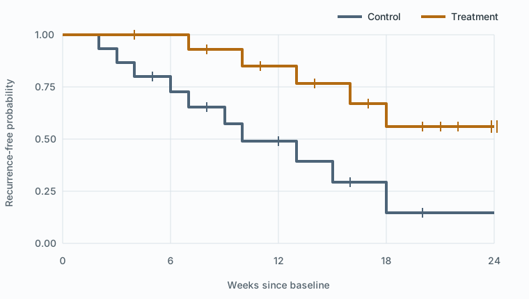
Ŝ(t) = product over event times ≤ t of [1 − events at that time ÷ participants at risk]Censoring reduces later risk sets but does not create a downward step
For example, the first control recurrence occurs at week 2 with all 15 control participants at risk. The estimate becomes 14/15 = .933. Recurrences cause vertical steps. Censoring marks where follow-up ends and removes that participant from later risk sets.
Review risk sets and selected estimates
| Week | Control at risk | Treatment at risk |
|---|---|---|
| 0 | 15 | 15 |
| 6 | 11 | 14 |
| 12 | 6 | 10 |
| 18 | 2 | 6 |
| 24 | 0 | 2 |
“At risk” means still under observation and recurrence-free immediately before that time. The risk sets become small late in follow-up, so the curve tails carry much less information than the early portions.
| Group | Participants | Recurrences | Censored | Median recurrence-free time |
|---|---|---|---|---|
| Control | 15 | 10 | 5 | 10 weeks |
| Treatment | 15 | 5 | 10 | Not reached |
- Control survival at week 10
- 0.4909
- Treatment survival at week 10
- 0.8512
- Control survival at week 18
- 0.1473
- Treatment survival at week 18
- 0.5586
The control curve first reaches or falls below .50 at week 10, so its estimated median recurrence-free time is 10 weeks. The treatment estimate remains above .50 through its final event time and subsequent censoring; its median is therefore not reached during observed follow-up. “Not reached” is not the same as “no median exists” or “the median is infinite.”
Compare the curves with the log-rank test
The log-rank test compares the observed number of events in each group with the number expected at the pooled event times under equal survival functions. It accumulates this comparison across follow-up while accounting for the changing risk sets.
- Control observed recurrences
- 10
- Control expected recurrences
- 5.6299
- Treatment observed recurrences
- 5
- Treatment expected recurrences
- 9.3701
- Log-rank statistic
- χ²(1) = 5.7976
- Two-sided p-value
- 0.0160
At α = .05, the synthetic data provide evidence against equal recurrence-free survival functions. The direction is understood from the curves and observed-versus-expected events: the treatment group has fewer recurrences than expected under the null, and its curve remains higher.
The p-value does not quantify the size of the separation. The ordinary log-rank output also does not provide a hazard ratio, an absolute risk difference at a chosen time with its uncertainty, or a covariate-adjusted treatment effect.
Assumptions and design checks
- Independent participants: each participant contributes one event or censoring time. Clustered participants require methods that reflect the cluster structure.
- Common, meaningful time origin: follow-up begins from the same defined point for both groups.
- Correct event coding: 1 means recurrence and 0 means right-censored. Reversing these codes changes the analysis completely.
- Non-informative censoring: conditional on the design and available information, censoring should not selectively remove participants because of an unobserved recurrence risk that the analysis ignores.
- Comparable event ascertainment: follow-up schedules and recurrence definitions should not systematically differ between groups.
- Curve comparison: the log-rank test is particularly responsive to persistent separation of the kind shown here. Strongly crossing curves may require a more carefully chosen estimand and method.
Reproduce the result in BioTabular
- Download the synthetic CSV and open the Kaplan–Meier survival calculator.
- Import the file. Keep
Participant_IDas the identifier,Groupas categorical, and bothFollow_up_weeksandEvent_statusas numeric. - Review the categorical order, then confirm the variable roles.
- Select
Follow_up_weeksas time,Event_statusas the event indicator, andGroupas the grouping column. - Run the analysis at α = .05. Confirm 30 included observations, 15 recurrences, 15 censored observations, control median 10, treatment median not reached, and log-rank χ²(1) = 5.798, p = .016.
- Inspect the curve, confidence bands, censoring marks, and risk sets before interpreting the comparison.
Interpret and report the result
During the observed 24-week period, the treatment group has a higher estimated probability of remaining recurrence-free. The evidence concerns the full unadjusted survival functions represented by these data. It does not prove proportional hazards, identify a biological mechanism, or rule out bias from censoring, event ascertainment, or study conduct.
“Thirty participants were followed for up to 24 weeks. Recurrence occurred in 10 of 15 control participants and 5 of 15 treatment participants; the remaining observations were right-censored. The Kaplan–Meier median recurrence-free time was 10 weeks in control and was not reached in treatment. Recurrence-free survival differed between groups in an unadjusted log-rank test, χ²(1) = 5.80, p = .016, with the treatment curve remaining above control during observed follow-up.”
A complete report should also define baseline, recurrence, censoring, administrative follow-up, analysis population, any competing events, and whether the comparison was prespecified.
Common mistakes this example avoids
- Analyzing follow-up time with a t-test and ignoring censoring.
- Treating censored participants as if they had the event at their last visit.
- Treating censoring as proof that a participant stayed recurrence-free forever.
- Reporting a median when the curve never reaches .50.
- Interpreting a log-rank p-value as a hazard ratio or effect size.
- Reading the sparse tail of a curve as precisely as its early portion.
- Using an ordinary Kaplan–Meier analysis when competing risks change the scientific question.
Limits of this worked example
The study is small, synthetic, unadjusted, and has no delayed entry, interval censoring, recurrent events, competing risks, site clustering, or time-varying covariates. BioTabular currently provides ordinary Kaplan–Meier estimates and a log-rank comparison. A real study may need a Cox model, restricted mean survival time, competing-risks methods, stratification, cluster-robust inference, or another prespecified analysis chosen for the estimand and design.
Related resources
Return to Which Statistical Test Should I Use? for the broader distinction between time-to-event outcomes and ordinary numeric outcomes. Compare this one-record-per-participant analysis with the longitudinal mixed-model worked example, where each participant contributes repeated numeric measurements rather than one event or censoring time.
References and further reading
- Kaplan and Meier (1958): Nonparametric estimation from incomplete observations
- Mantel (1966): Evaluation of survival data and two new rank order statistics
- NIST/SEMATECH e-Handbook of Statistical Methods
- American Statistical Association statement on statistical significance and p-values
BioTabular’s editorial approach and scope explain how these educational resources are prepared and what they do not replace.