WORKED EXAMPLE
Fisher’s Exact Test Worked Example: A Sparse 2×2 Table
Follow a two-sided Fisher exact test from participant-level binary data through the observed 2×2 table, expected counts, exact probability, effect estimates, BioTabular setup, interpretation, and reporting language.
Published by BioTabularPublished and reviewed: October 26, 2026
This teaching example uses synthetic values. It is not clinical evidence and does not claim that a real treatment prevents adverse events.
Research question and study design
Suppose a randomized pilot study records whether each participant experiences a specified adverse event during follow-up. Eight participants receive treatment and ten receive control. The research question is: Are treatment assignment and adverse-event status associated in the source population?
- Observational unit
- The participant.
- Group structure
- Each participant belongs to treatment or control, never both.
- Outcome
- A binary classification: Event or No event.
- Table structure
- Two group levels by two outcome levels: a 2×2 table.
- Comparison direction
- Treatment relative to control; a negative risk difference means fewer observed treatment events.
- Starting method
- A two-sided Fisher exact test when the 2×2 expected counts are sparse.
The synthetic participant-level dataset
Every row represents one independent participant. The group and outcome categories are mutually exclusive, and there are no missing records. The file retains the rows that produce the count table so the design can be checked before analysis.
| Participant | Group | Adverse event |
|---|---|---|
| C01 | Control | Event |
| C02 | Control | Event |
| C03 | Control | Event |
| C04 | Control | Event |
| C05 | Control | Event |
| C06 | Control | Event |
| C07 | Control | Event |
| C08 | Control | No event |
| C09 | Control | No event |
| C10 | Control | No event |
| T01 | Treatment | Event |
| T02 | Treatment | No event |
| T03 | Treatment | No event |
| T04 | Treatment | No event |
| T05 | Treatment | No event |
| T06 | Treatment | No event |
| T07 | Treatment | No event |
| T08 | Treatment | No event |
Privacy note: this downloadable file is synthetic. When imported into the Workspace, BioTabular processes it in browser memory during the active page session rather than uploading the rows to BioTabular.
Build the observed 2×2 table
Counts—not percentages alone—form the input to Fisher’s test. Order the rows as Treatment then Control and the columns as Event then No event so every later effect direction stays explicit.
| Group | Event | No event | Total |
|---|---|---|---|
| Treatment | 1 | 7 | 8 |
| Control | 7 | 3 | 10 |
| Total | 8 | 10 | 18 |
The observed event risks are 1/8 = 12.5% for treatment and 7/10 = 70.0% for control. The descriptive treatment-minus-control risk difference is −57.5 percentage points, and the descriptive risk ratio is 0.179.
Why Fisher’s exact test is primary
Under independence, an expected count is (row total × column total) ÷ overall total. The expected treatment/event count is (8 × 8) ÷ 18 = 3.5556. The complete expected table is:
- Treatment / Event
- 3.5556
- Treatment / No event
- 4.4444
- Control / Event
- 4.4444
- Control / No event
- 5.5556
- Expected cells below 5
- 3 of 4
- Complete observations
- 18; omitted 0
Three expected counts are below five, so the ordinary chi-square large-sample approximation is questionable here. BioTabular therefore presents Fisher’s exact test as the primary result for this sparse 2×2 table. The method choice follows the table and design, not whichever method gives a preferred p-value.
Calculate the exact probability
Fisher’s test conditions on the observed row and column totals. With those margins fixed, the treatment/event cell determines the remaining three counts. Under the null model, the probability of exactly one event among the eight treatment participants is hypergeometric:
P(X = 1) = choose(8, 1) × choose(10, 7) ÷ choose(18, 8)Observed-table probability = 0.02193885
For BioTabular’s two-sided definition, probabilities are added for all fixed-margin tables whose probability is no greater than the observed table’s probability. The resulting two-sided Fisher exact p-value is 0.02481832.
Inspect the observed percentages
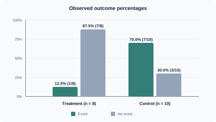
The plot describes this sample; it does not replace the test or establish causation. Because the denominators differ, compare within-group percentages rather than raw event counts alone.
Assumptions and practical checks
- Independent observations: each participant contributes to one cell only.
- Mutually exclusive categories: group and outcome definitions must be unambiguous.
- Count data: cells contain non-negative whole-number counts, not percentages or means.
- Prespecified outcome: repeatedly selecting outcomes or subgroups after viewing results changes the error context.
- Appropriate design: ordinary Fisher and chi-square tests do not account for matching, repeated observations, or clustering.
“Exact” refers to the conditional probability calculation. It does not correct measurement error, selection bias, missing data, confounding, protocol deviations, or a design that fails to support the intended interpretation.
Reproduce the result in BioTabular
- Download the synthetic CSV and open the categorical-association calculator.
- Import the file. Keep
Participant_IDas the identifier and bothGroupandAdverse_Eventas categorical. - Before confirming roles, move Treatment above Control in the Group order. Keep Event above No event.
- Confirm the variable roles. Select
Groupas the first categorical variable andAdverse_Eventas the second. - Run chi-square / Fisher and keep α = 0.05 for this example.
- Confirm 18 complete rows, the Treatment-first observed table, three expected cells below five, and Fisher exact p = .025 after display rounding.
- Use the grouped-bar Plot Studio handoff to inspect counts or within-group percentages.
Interpret the result
At the prespecified 0.05 level, the two-sided Fisher p-value is below alpha. Under the conditional null model, the sparse table provides evidence of an association between group and adverse-event status. The observed direction favors fewer events under treatment.
The p-value does not measure effect size. The risk difference, risk ratio, or odds ratio supplies that scale, while an interval communicates precision. Here the estimates are dramatic but uncertain. A real causal interpretation would additionally depend on randomization integrity, adherence, outcome ascertainment, missing data, and whether this analysis was prespecified.
Reporting example
“An adverse event occurred in 1 of 8 treatment participants (12.5%) and 7 of 10 control participants (70.0%), a descriptive risk difference of −57.5 percentage points. Because the 2×2 table was sparse, a two-sided Fisher exact test was used (p = .0248). The conditional odds-ratio estimate was 0.074 (95% exact CI 0.0012 to 0.968). The small sample produced substantial uncertainty, so the effect magnitude should be interpreted cautiously.”
A complete report should also describe allocation, eligibility, outcome definitions, missing-data handling, follow-up, protocol deviations, and whether the outcome and analysis were prespecified.
Fisher exact is not Wilcoxon exact
The word exact describes how a null distribution or p-value is calculated; it does not identify the outcome type. Fisher’s exact test analyzes counts in a contingency table formed by categorical variables. An exact Wilcoxon rank-sum or signed-rank procedure analyzes ranks from numeric or ordinal observations. These are different tests for different data structures and are not interchangeable.
Common mistakes this example avoids
- Testing percentages without their underlying counts.
- Looking only at observed counts instead of expected counts when assessing sparsity.
- Reversing group or outcome order while retaining effect wording for the original direction.
- Reporting only the p-value without counts, percentages, an effect estimate, and uncertainty.
- Treating repeated or matched observations as independent.
- Interpreting “exact” as proof that the study or scientific conclusion is exact.
Limits of this worked example
This illustration has two independent groups, one binary outcome, no missing observations, and no covariate adjustment. Paired binary outcomes may call for McNemar’s test; matched case-control sets may call for conditional logistic regression; clustered or repeated observations need a dependence-aware model; and larger sparse tables may require another exact or simulation-based approach.
Related resources
Read Chi-square vs. Fisher’s Exact Test for the broader method choice. Use Which Statistical Test Should I Use? for other outcome types, or compare the continuous-outcome independent t-test worked example.
References and further reading
- R documentation: Fisher’s Exact Test for Count Data
- R documentation: Wilcoxon Rank Sum and Signed Rank Tests
- Statistical notes for clinical researchers: Chi-squared test and Fisher’s exact test
- Foundations of statistical inference with 2×2 tables
- NIST/SEMATECH e-Handbook of Statistical Methods
- American Statistical Association statement on statistical significance and p-values
BioTabular’s editorial approach and scope explain how these educational resources are prepared and what they do not replace.